Model Name Matrix Referral Specific Gravity: Valid for SRD
1. What it does?Uses regression to compute TCD and SG using input product-density datasets
2. ApplicationPetroleum/Petrochemicals Industry.
3. MathsSpecific gravity is calculated by a Process of interpolation and extrapolation between a matrix of known density and temperature reference points.

Figure 1. Matrix of known density and temperature.
This to determinate the liquid density at a specified base temperature different to the inline temperature. Temperature-density data is converted into coefficients for calculation of temperature compensated density at a reference temperature.

Figure 2. Temperature-Density to compensate density
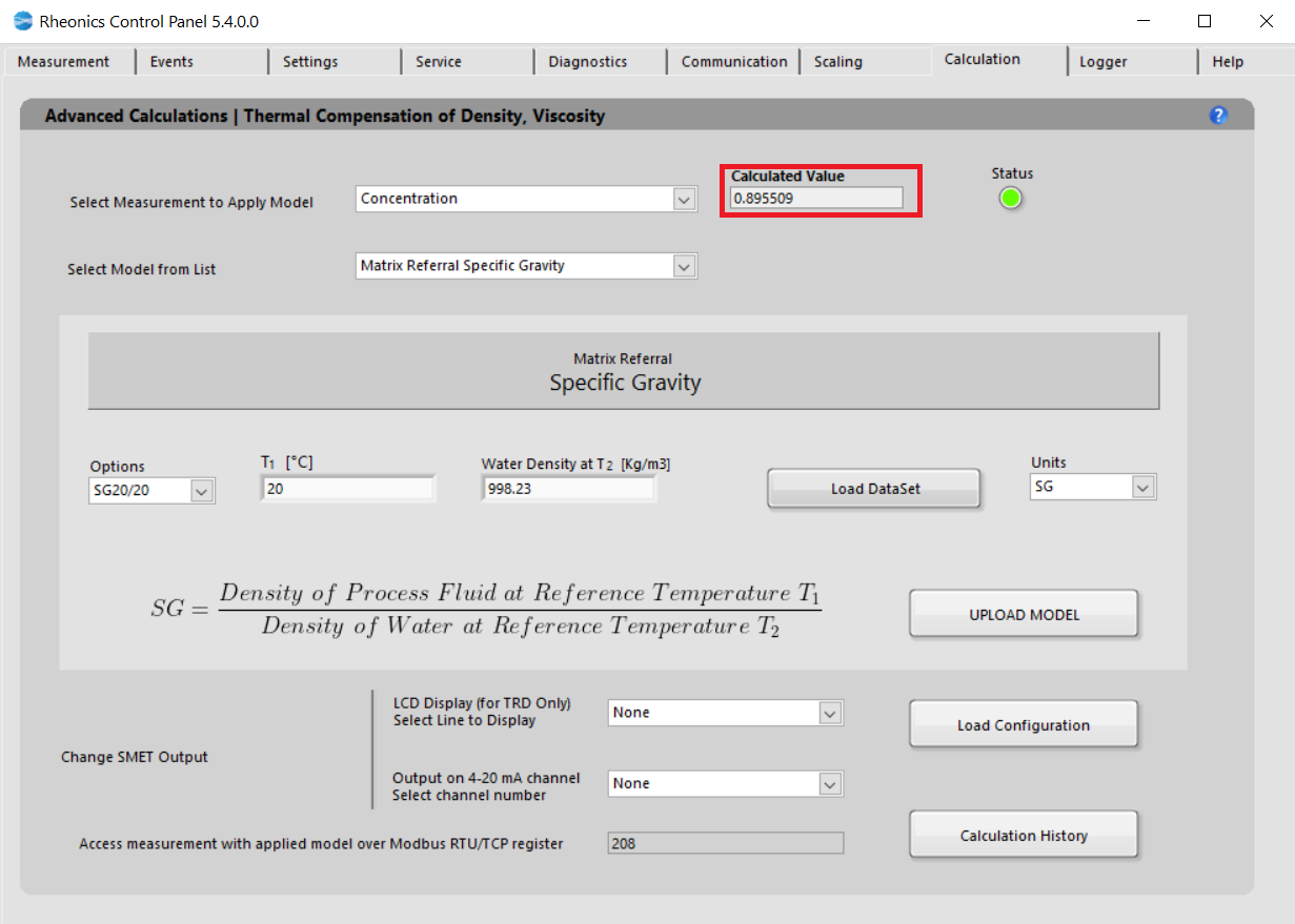
4. How to load models into the SME?Calculation tab allows to configure the SME to run mathematical models for Viscosity, Density and Concentration.

Figure 3. Calculation tab for Specific Gravity model
The following steps are to load the models into SME:
- In the Dropdown list “Select Measurement to Apply Model” select. That will modify the “Select Model from List” dropdown menu values. Select Measurement application (Concentration)
- In “Select Model from list” select the model you would like to use for the specific parameter. When you select the model, you will get more information about the specific equation used and the coefficients you will need to apply that model. Select “Matrix Referral Specific Gravity”.
- Select Specific gravity reference temperature and density from the dropdown list. Four (4) options available: SG20/20(Water density at 20°C), SG20/4(Water density at 4°C), and SG60/60(Water density at 60°F). Red square box parameter cannot be modified unless Custom model is selected.
- “Load Dataset” button, this operation is crucial to get correct measurement for Specific Gravity measurement so as density and temperature to be measurement from the process mut be within this table. Dataset table must cover at least the following instances:
- Five reference temperatures (at least)
- The density for each of four product types at the five reference temperatures
- The base temperature, which must be one of the five reference temperature

Figure 4. 20 datapoint set.
4.4. Dataset for a generic 20 datapoint set, first column is for temperature. The rest of the columns should be each for a product "P", and the densities of that product at the different temperatures.
4.5. Import: Select dataset from an .csv sheet

Figure 5. Selecting dataset
4.5. Export: Export current table to .csv
4.6. "Tk1, Tk2" button to create the coefficients that will be used on the model.
4.7. Calculated Tk coefficients by internal model.
4.8. "Load Tks & Close" button to load these coefficients into the model
5. Uploading the Mathematical ModelClick “Upload Model” to load the model settings into SME. The button should turn GREEN for a couple of seconds if the action was successful or turn RED if the operation was Rheonics Control Panel Software unsuccessful. This action will refresh the values for the Uncompensated and Compensated indicators. Here you can verify if the model is calculating the expected values. If not, you can correct and repeat the process.
5.1. Click “Load Configuration” to update the display and channel configurations in SME.
5.2. LCD Display
Select the line to display the parameter:

Figure 6. Selecting read line for LCD display
5.3. Changes can be verified in “Communication” Tab

Figure 7. Communication tab has loaded concentration parameter
5.4. Analog outputs
Select analog channel to send data, this can be verified in “Service” Tab

Figure 8. Selecting analog output channel
5.5. Modbus TCP/IP register
Measurement can always be accessed at the register address that is displayed.

5.6. “Calculation History” button allows you to open a file where the last uploaded models and coefficients for these models are stored. This is for user reference.