
| What products are involved? This article is based on the use of RCP (Rheonics Control Panel) connected to the SME (Smart Module Electronics) from SRV, SRD, DVP and DVM. It therefore applies to any of these Rheonics sensors. What is the purpose of this article? To explain the process for obtaining a temperature-compensated viscosity when the fluid shows a second-degree polynomial trend. Typical applications include thermal oils and molten salts. |
Temperature Compensated Viscosity – Polynomial Model
1. Temperature compensated viscosity
Viscosity, defined as the ratio of shear stress to shear rate, is an important fluid property with an increasing presence in monitoring processes and control systems.
Viscosity is affected by temperature and pressure. For most liquids, viscosity decreases with temperature, whereas it increases for gases. An increase in pressure typically increases viscosity, which is only relevant for high-pressure applications.
In most cases, the goal is to monitor fluid viscosity at a constant reference temperature. If the process temperature isn't constant, it adds an additional source of error to the control system. To remove the temperature dependence from the fluid's viscosity and truly monitor its consistency, the temperature-compensated viscosity is introduced.
To compensate for temperature effects, a mathematical model is needed, based on either an exponential or a polynomial function.
2. Math model
The SRV and SME together form a powerful tool for measuring inline viscosity and temperature. Using mathematical models, temperature-compensated measurements can be obtained.
Below is the mathematical formula for the viscosity polynomial model used in RCP (Rheonics Control Panel).

Equation 1. Viscosity Polynomial Model.
Where:
- ηcomp — Compensated viscosity, calculated by the SME.
- ηL — Live viscosity, read by the SME.
- X1 and X2 — Coefficients, added by the user.
- T — Temperature, read by the SME.
- Tref — Reference temperature: the temperature around which the SME will compensate the readings. Defined and entered by the user.
Along with the reference temperature, the reference viscosity (viscosity at Tref) is also relevant for the calculations explained below.
3. Checking the data
Take viscosity readings across the normal operating temperature range, then extend a bit further with higher and lower temperatures. Once enough data is available to see the polynomial behavior, define the reference temperature.
For this example, 20 °C (highlighted in blue) is used as the typical set-temperature of the process line. Additional measurements should extend a bit beyond the expected temperature range.
The following steps outline the correct procedure for data analysis:
3.1. Select the reference temperature and viscosity from the test data (highlighted in blue in Table 1). Here, a correlation is created at 20 °C where a viscosity of 1 mPa·s is expected.
| Temperature (°C) | Viscosity (mPa·s) |
| 30 | 0.75 |
| 25 | 0.85 |
| 20 | 1 |
| 15 | 1.1 |
| 10 | 1.25 |
| 5 | 1.5 |
| 0 | 1.75 |
Table 1. Data points from inline measurements.
3.2. Plot Viscosity vs Temperature to study the behavior of the data. In this scenario, the data can be represented by a second-order polynomial curve.
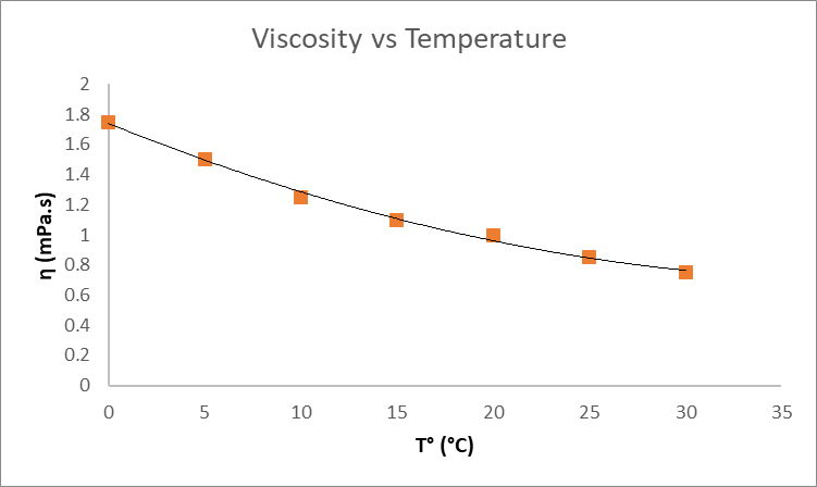
Figure 1. Plot chart Viscosity vs Temperature.
3.3. Calculate the ratio between the compensated (reference) viscosity and the measured viscosity by dividing the two.
| V' = (Compensated Viscosity / Viscosity) @20°C | Result |
| V' = (1/0.75) | 1.3333 |
| V' = (1/0.85) | 1.1764 |
| V' = (1/1) | 1.0000 |
| V' = (1/1.1) | 0.9091 |
| V' = (1/1.25) | 0.8000 |
| V' = (1/1.5) | 0.6667 |
| V' = (1/1.75) | 0.5714 |
Table 2. Compensated viscosity calculation table.
3.4. Calculate the difference between measured and reference temperature by subtracting them.
| T' = T - Tref | Result |
| T' = 30-20 | 10 |
| T' = 25-20 | 5 |
| T' = 20-20 | 0 |
| T' = 15-20 | -5 |
| T' = 10-20 | -10 |
| T' = 5-20 | -15 |
| T' = 0-20 | -20 |
Table 3. Variation from the reference temperature.
3.5. Plot V' (Comp. Visc./Visc. @20°C) vs T' (T–Tref) and use a second-order polynomial trendline to find the X1 and X2 values, or run a regression analysis to find the coefficients.
| V' | T' |
| 1.3333 | 10 |
| 1.1764 | 5 |
| 1.0000 | 0 |
| 0.9091 | -5 |
| 0.8000 | -10 |
| 0.6667 | -15 |
| 0.5714 | -20 |
Table 4. Data points for viscosity and temperature referenced to known values.
A graphing tool is used to create a trendline from the points obtained; it can also show the trendline equation.
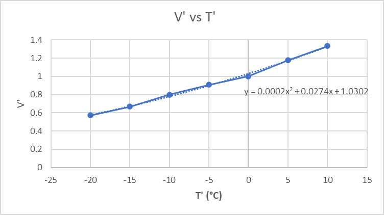
Figure 2. Plot chart V' vs T'.
The trendline equation from Figure 2 is compared against Equation 1, accepting the leading coefficient value of 1.0302, rounded to 1.
This gives:
X1 = 0.0274 and X2 = 0.0002
With:
Tref = 20 °C
With these input parameters set on the SME through RCP, the temperature-compensated viscosity looks like the graph in Figure 3.
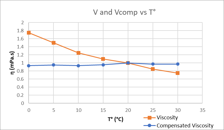
Figure 3. Expected results when applying the mathematical model.
4. How to load models into the SME
The Calculation tab in RCP allows configuring the SME to run mathematical models for viscosity, density, and concentration. Expert Mode needs to be enabled for this.
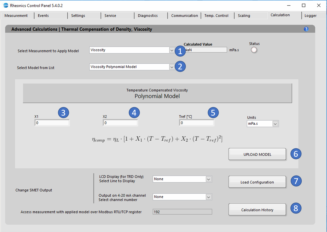
Figure 4. Calculation tab for the polynomial model of viscosity.
The following steps are needed to load the model into the SME:
- In the "Select Measurement to Apply Model" dropdown, viscosity should be the default parameter. If not, select it from the list.
- In "Select Model from list", select the model to use for the parameter. Selecting a model shows more information about the equation used and the coefficients required. Select "Viscosity Polynomial model".
- Input the calculated X1 coefficient. For this example, 0.0274.
- Input the calculated X2 coefficient. For this example, 0.0002.
- Input the reference temperature used to find the model coefficients. In this example, 20 °C.
- Click "Upload Model" to load the model settings into the SME. The button turns green briefly if successful, or red if unsuccessful. This refreshes the uncompensated and compensated indicators so the model's output can be verified — correct and repeat the process if needed.
- Click "Load Configuration" to update the display and channel configurations in the SME.
4.1. LCD Display
For the SME-TRD, compensated viscosity values can be shown on the display. Select the line to display the parameter:
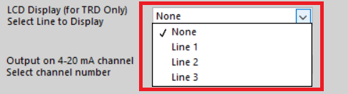
Figure 5. Selecting read line for LCD display.
Changes can be verified on the "Communication" tab.
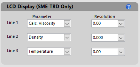
Figure 6. The communication tab with the loaded parameter.
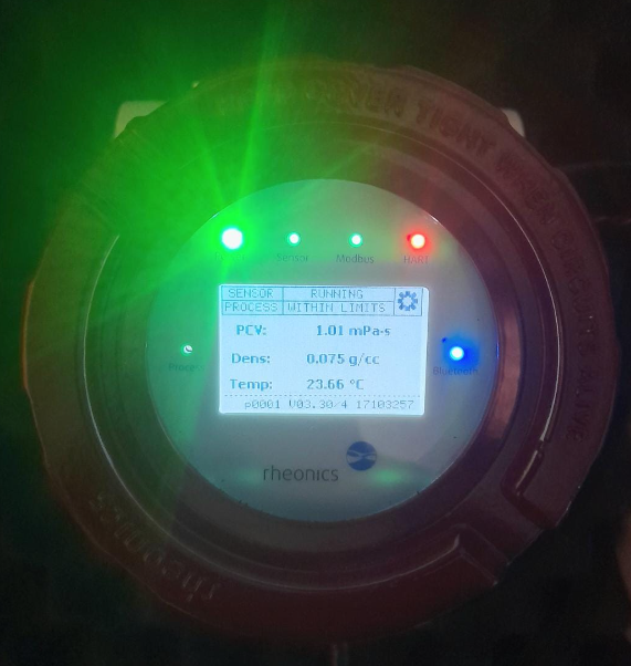
Figure 7. Parameters loaded into the SMET-TRD.
It is also possible to see and use the calculated data over 4–20 mA channels, Profinet, Modbus, and others. See Using calculated data from SME.
References/Further information
Temperature Compensated Viscosity – Exponential Model
Using Calculated Data from SME
RCP Manual — Rheonics Control Panel software, used to acquire data from Rheonics sensors and to configure the sensor.
SRV Product Information
SRD Product Information
DVP Product Information
DVM Product Information