What products are involved?
This article is based on using multiple Rheonics sensors and the USR-W610 to send various sensor data through Wi-Fi to an MQTT Broker using Node-RED and visualize it remotely via Ignition SCADA.

What is the purpose of this article?
This article demonstrates how to integrate the USR-W610 RS232/RS485 to Wi-Fi & Ethernet Converter with multiple Rheonics sensors simultaneously in Ignition SCADA.

TABLE OF CONTENTS

• 1. Overview
• 2. USR-W610 Setup
• 3. Sensor Module Electronics (SME) Configuration
• 4. Node-RED
  • 4.1. MQTT Topic Naming Convention
• 5. Configuring Ignition SCADA MQTT
• 6. Visualization in Ignition Designer
• 7. References

1. Overview

The remote visualization of multiple sensor data is utilized for fluid monitoring and diagnostics across different locations. This section demonstrates how to connect and publish data from several Rheonics sensors using the USR-W610 to connect to a Wi-Fi network and send the data through Node-RED to an MQTT broker. The following diagram presents the architecture with multiple sensors using the USR-W610 converter.

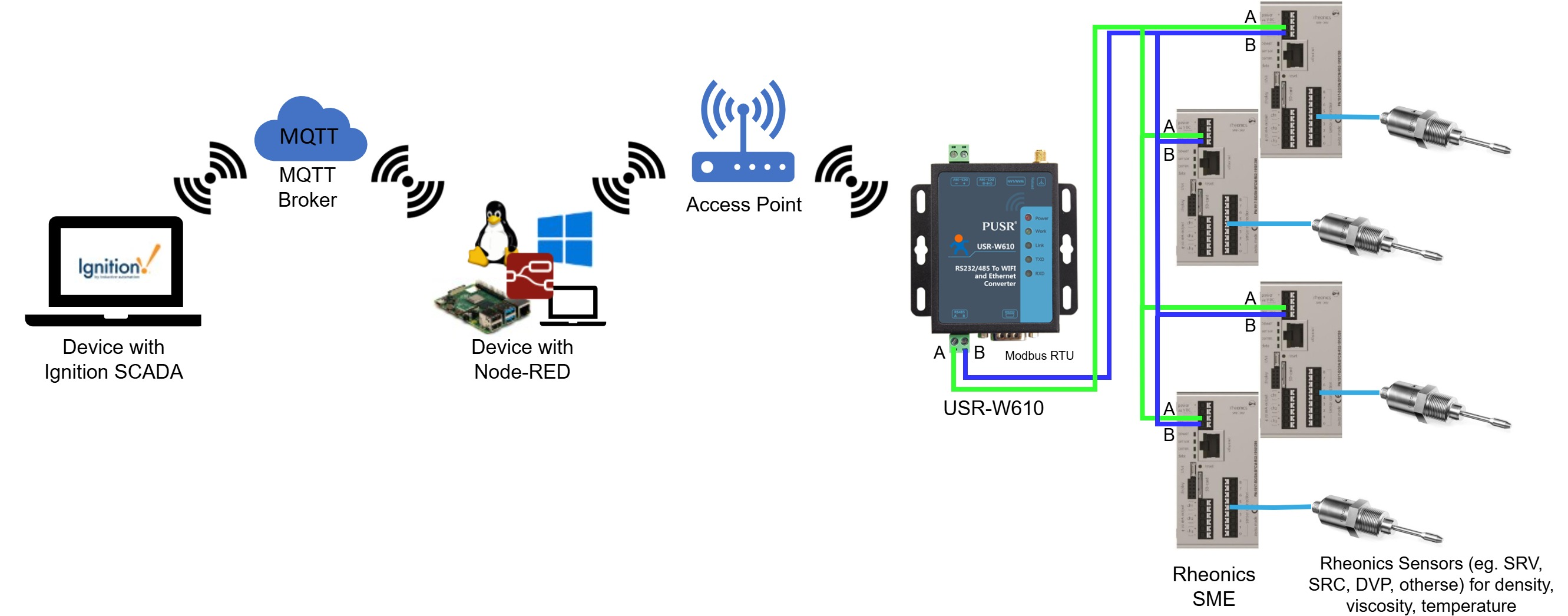Figure 1: Architecture of multiple Rheonics sensors, USR-W610, Node-RED and Ignition SCADA integration

2. USR-W610 Setup

The USR-W610 module is used to send data to a Wi-Fi network. In this case, the device is configured as STA, so it is connected to the same Wi-Fi network as the device with Node-RED.

To see more information about the device setup refer to Connecting Rheonics Sensors to Wi-Fi Networks using USR-W610

3. Sensor Module Electronics (SME) Configuration

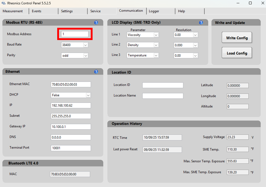
Each SME needs to have a different Modbus Address, in this case 4 SMEs are used to read 4 sensors, so the addresses are configured differently. This can be configured in the Rheonics Control Panel. Refer to the Modbus RTU Manual found in Manuals 

4. Node-RED

To learn the basic steps for setting up Node-RED and using the modules mentioned in this article, visit the Node-RED Setup and MQTT for Rheonics Sensors

To integrate more sensors in Node-RED, add a new Modbus client for each SME, assigning each its respective Modbus Address. In this example, parameters from three SRV sensors and one SRD sensor are read, each configured with the same IP address configured in the USR-W610 but with a different Unit-ID. Each Modbus-Read node in Node-RED is paired with a corresponding MQTT-out node to publish the sensor data.

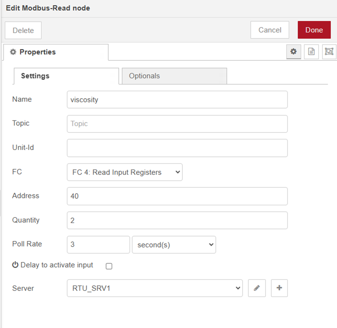
2. Configure the node with the following to read viscosity. The rest of the input parameters can be found in Modbus Input Registers

• Name: e.g. viscosity
• FC: FC4: Read Input Registers
• Address: 40
• Quantity: 2
• Poll rate: 3

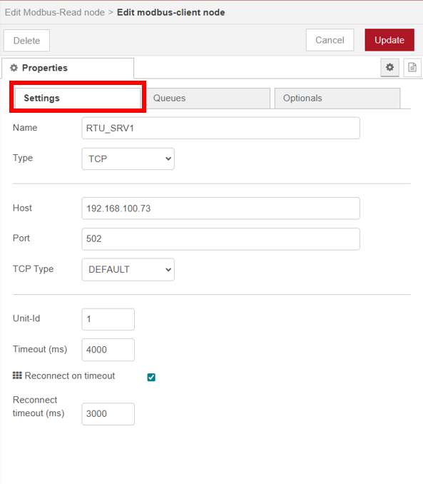
3. On the Modbus-Read node, click on the Server field and press the plus to add a new Modbus client. In this case, it corresponds to one of the SME. In the Setting Tab, configure the following:

• Type: TCP
• Host: IP established in the USR-W610
• Port: 502 (default)
• Unit ID: Modbus Address of the SME
• Timeout: 4000
• Reconnect on timeout:✅
• Reconnect timeout (ms): 3000

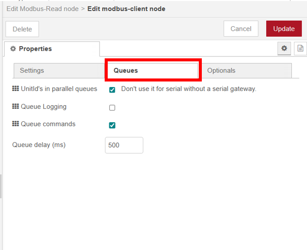
4. On the Queues Tab, configure as follows. This is to avoid overwhelming the USR-W610 and read the measurements correctly.

• UnitId’s in parallel queues: ✅
• Queue commands: ✅
• Queue delay (ms): 500

4.1. MQTT Topic Naming Convention

To learn how to send Rheonics sensor data to an MQTT broker using Node-RED, refer to Integrating Rheonics Sensors with Node-RED and MQTT for Remote Data Access

To keep topics organized, follow a structured naming scheme. Ensure each sensor’s data is published to a unique MQTT topic to prevent conflicts and to make data handling easier on the Ignition Designer side. For this example, the format used is the following:

• SRV1
  • viscosity: srv1/viscosity
  • density: srv1/density
  • temperature: srv1/temperature
• SRV2
  • viscosity: srv2/viscosity
  • density: srv2/density
  • temperature: srv2/temperature
• SRV3
  • viscosity: srv3/viscosity
  • density: srv3/density
  • temperature: srv3/temperature
• SRD
  • viscosity: srd/viscosity
  • density: srd/density
  • temperature: srd/temperature
  • kinviscosity: srd/kinviscosity

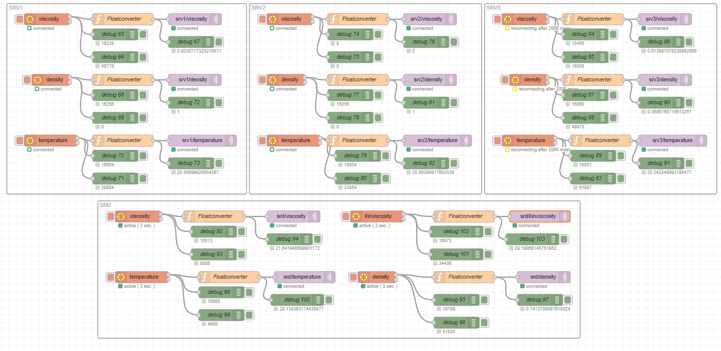Figure 7: Node-RED flow with multiple sensors

5. Configuring Ignition SCADA MQTT

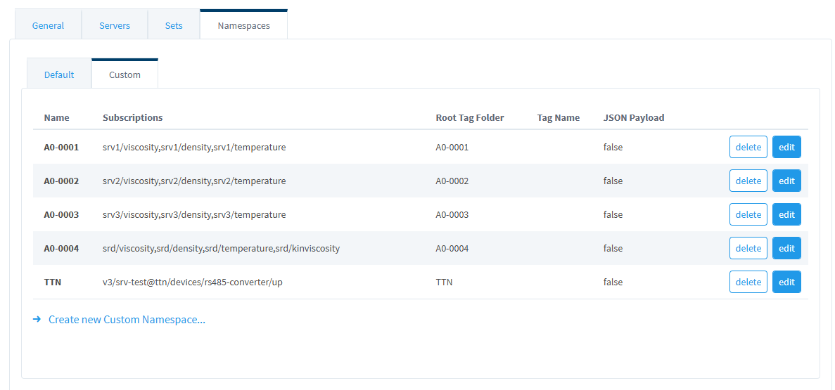
In Ignition SCADA, each SME can be linked to its custom namespace within the MQTT Engine module. This can help organize data by sensor and ensure clear identification across the interface.

• Name: For this example, each sensor’s serial number was used as the namespace name and as the Root Tag Folder name.
• Subscriptions: Assign the MQTT topics to each namespace based on the naming structure used in Node-RED.

This image displays the MQTT Engine’s configuration, showing how each sensor’s topics are grouped into their namespace.

6. Visualization in Ignition Designer

To learn how to connect Ignition SCADA to a MQTT broker to visualize Rheonics sensor data refer to Using Ignition SCADA to Visualize Rheonics Sensor Data via MQTT

Using the Rheonics templates available on Ignition Exchange, sensor data can be easily visualized. For this example, the existing display template was modified to have more SRV displays available to correctly assign each display to its respective tag.

The following figure shows the Tag Browser in Ignition Designer, where the sensor values are grouped under each namespace created previously, corresponding to each SME.

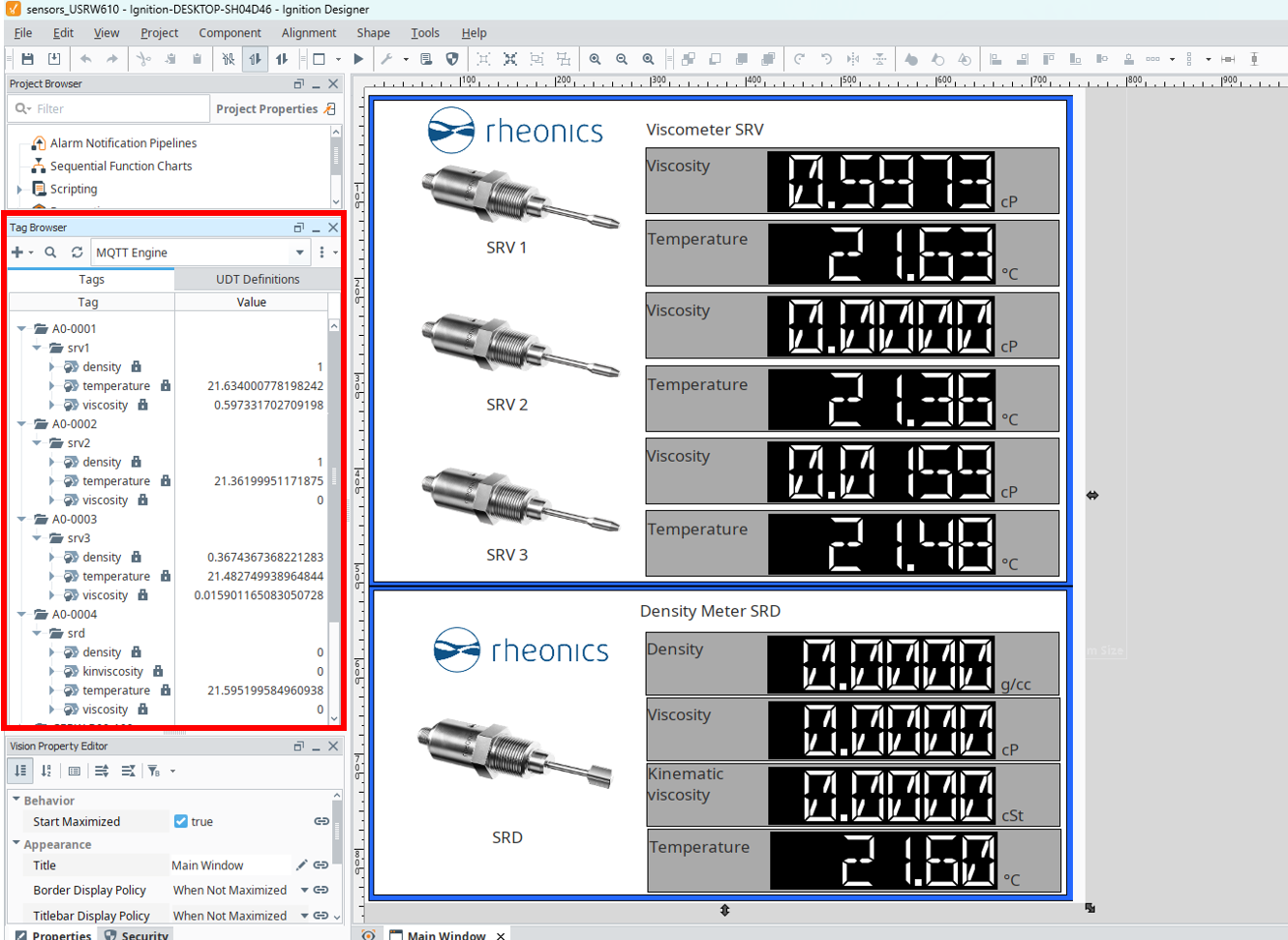Figure 9: Tag Browser in Ignition Designer

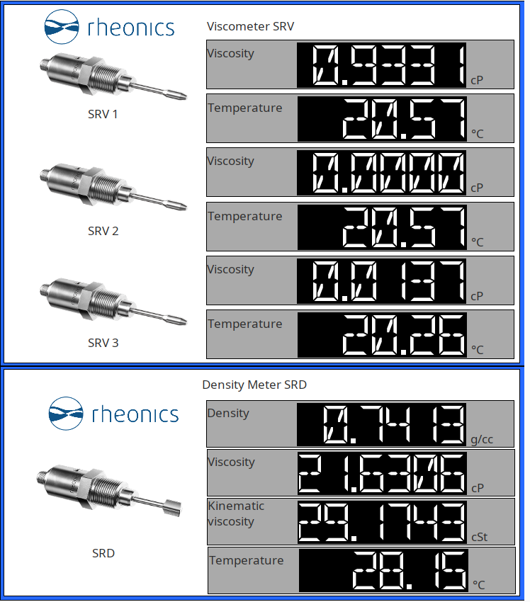
After assigning each value correctly to each display, the final view in Ignition Designer would look like the following figure.

7. References

• Connecting Rheonics Sensors to Wi-Fi Networks using USR-W610
• Manuals
• Node-RED Setup and MQTT for Rheonics Sensors
• Modbus Input Registers
• Integrating Rheonics Sensors with Node-RED and MQTT for Remote Data Access
• Using Ignition SCADA to Visualize Rheonics SME Data via MQTT