
What products are involved?
SME – Sensor Module Electronics | SRV – Inline Viscosity Meter | SRD – Inline Density & Viscosity Meter
What is the purpose of this article?
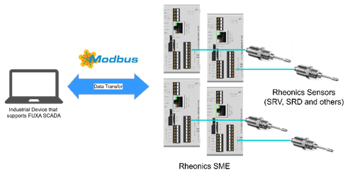
This article describes the integration of Rheonics Sensor Module Electronics (SME) via Modbus RTU with FUXA SCADA software. The goal is to enable communication between the SME and a web-based SCADA system.
| Short answer: Connect the Rheonics SME to FUXA SCADA using the Modbus RTU connection type, add the sensor parameters as variables using their register addresses, then build a real-time dashboard in the FUXA Editor using charts and controls to visualize the incoming values. |
TABLE OF CONTENTS
1. Overview
A web-based SCADA/HMI system enables real-time monitoring, control, and visualization of industrial processes through standard web browsers, allowing remote access from multiple devices without requiring specialized client software. By integrating industrial controllers, sensors, and IoT devices through widely adopted communication protocols, these systems provide essential functionalities such as live data visualization, historical data logging, alarm management, and event notifications.
In this case, FUXA SCADA is used. This software supports industrial communication standards such as Modbus RTU, Modbus TCP, MQTT, OPC UA, Siemens S7, and EtherNet/IP, enabling connectivity with field devices, including viscosity sensors and automated control systems.
This interoperability facilitates reliable data acquisition, process supervision, and performance analysis, making such systems particularly valuable in the food, chemical, pharmaceutical, and manufacturing sectors, where accurate viscosity monitoring is essential for maintaining product quality and operational stability.
2. FUXA SCADA
2.1 Communication Protocols
FUXA SCADA supports the following list of communication protocols through a Node.js-based server environment (Table 1), enabling integration with a wide range of industrial controllers, sensors, and automation devices. The platform operates on Windows, Linux, and Raspberry Pi/ARM architectures and is accessible through standard web browsers. Some protocols may require additional components, such as the node-snap7 library for Siemens S7 communication, while installation on Linux can present additional configuration challenges depending on the Node.js version used.
Table 1: Supported Communication Protocols
| Protocol | Requirements | Main Restrictions |
|---|---|---|
| Modbus RTU/TCP | Modbus-compatible PLC, sensor, or controller with RS-485 or TCP/IP connectivity. | Limited only by standard Modbus addressing constraints. |
| Siemens S7 | Siemens S7-200/300/400/1200/1500 PLC communicating via Ethernet. | Requires absolute addressing; maximum frame size of approximately 960 bytes, 255 variables per request, and 64 messages per connection; TCP/IP communication must be enabled in TIA Portal. |
| OPC UA | OPC UA-enabled device or third-party OPC UA server. | Subject to standard OPC UA security and encryption requirements. |
| BACnet IP | BACnet IP-compatible devices. | No significant protocol-specific restrictions. |
| MQTT | MQTT broker and MQTT-enabled devices. | Limited by standard MQTT topic and payload constraints. |
| EtherNet/IP | Allen-Bradley PLCs with EtherNet/IP support. | No documented protocol-specific restrictions. |
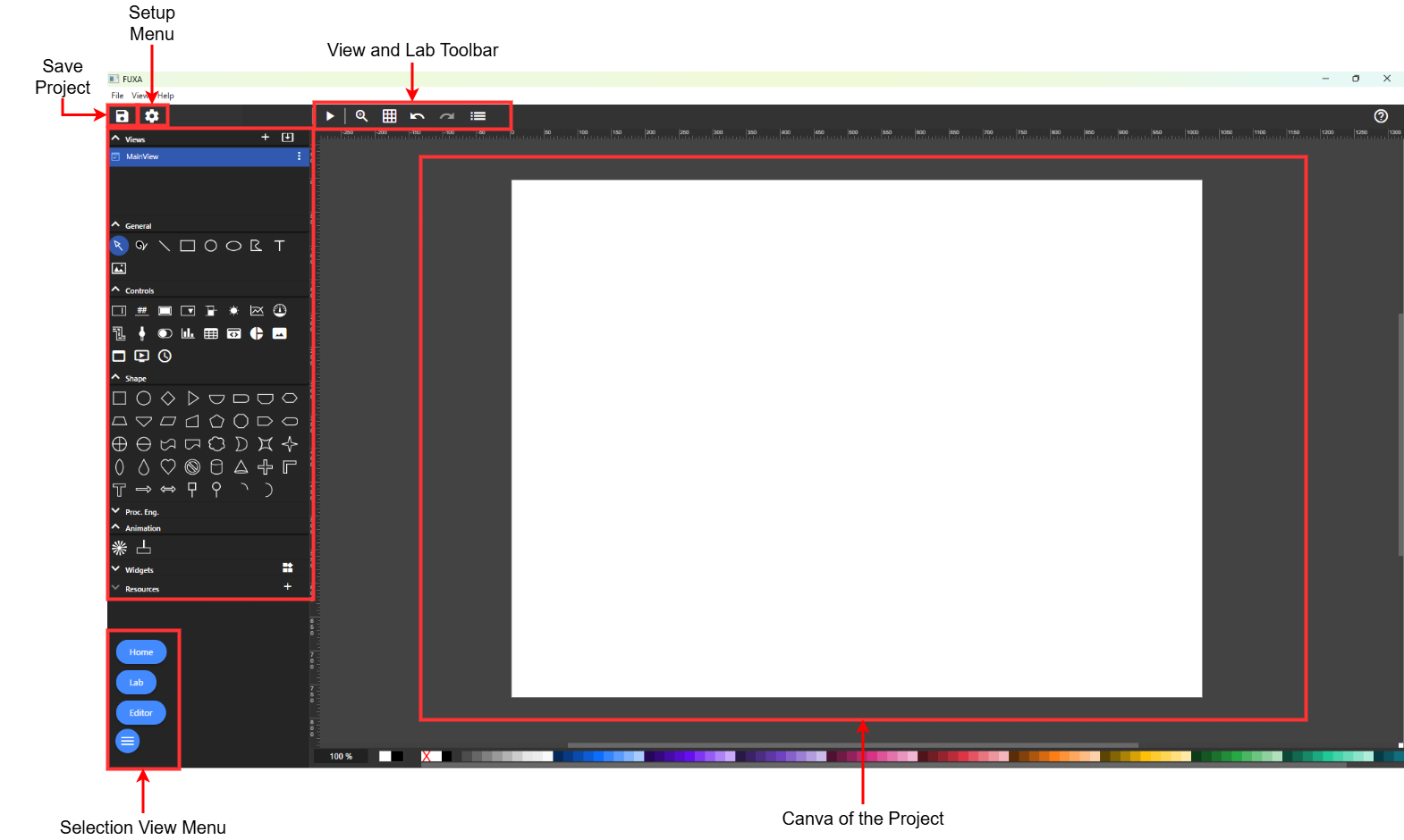
Figure 2: Main Screen of FUXA SCADA.
3. Integration with Rheonics SME
3.1 Connecting via Modbus RTU
Although the Rheonics SME can work with different communication protocols, the tests described in this article use the Modbus RTU protocol via a serial communication port using an adapter.
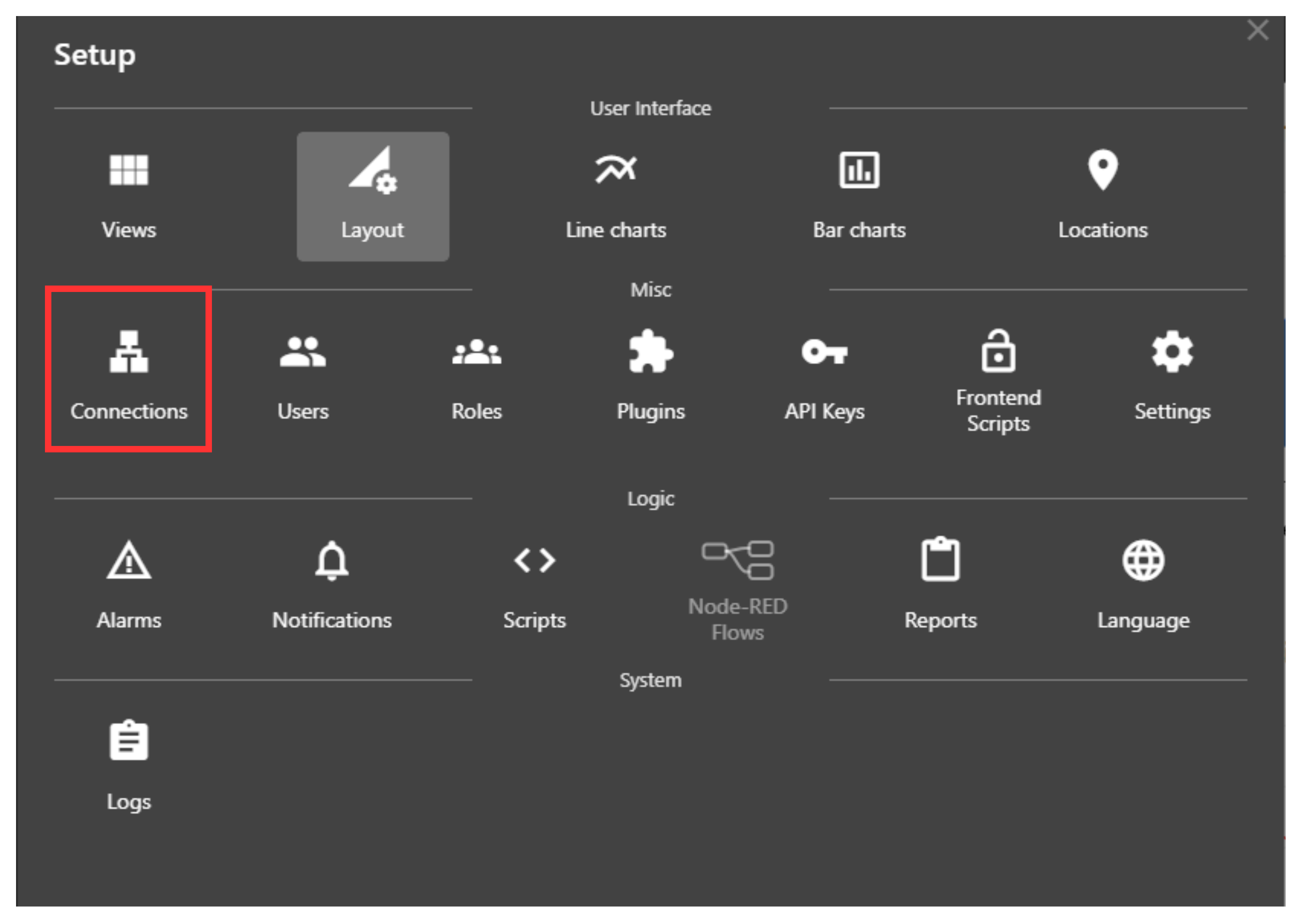
- Click on the Setup Menu and add a new connection in the Connection settings menu and choose Modbus RTU.
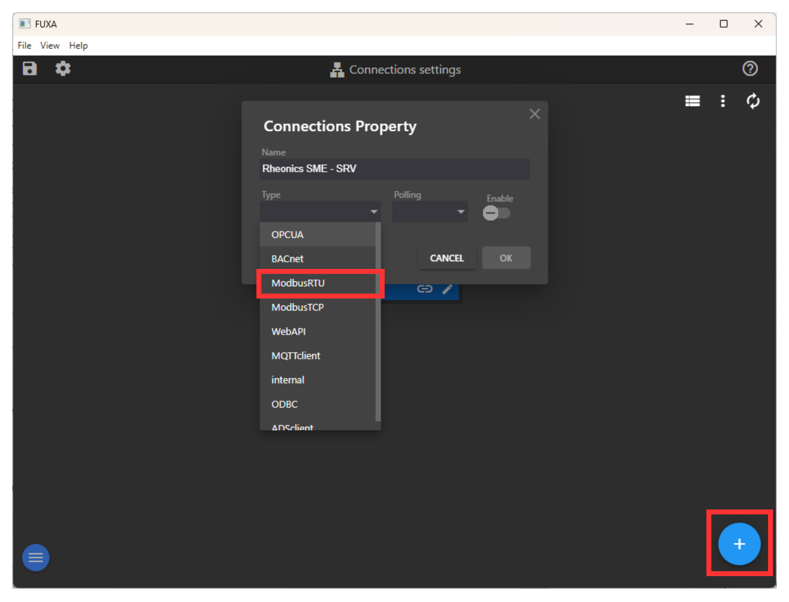
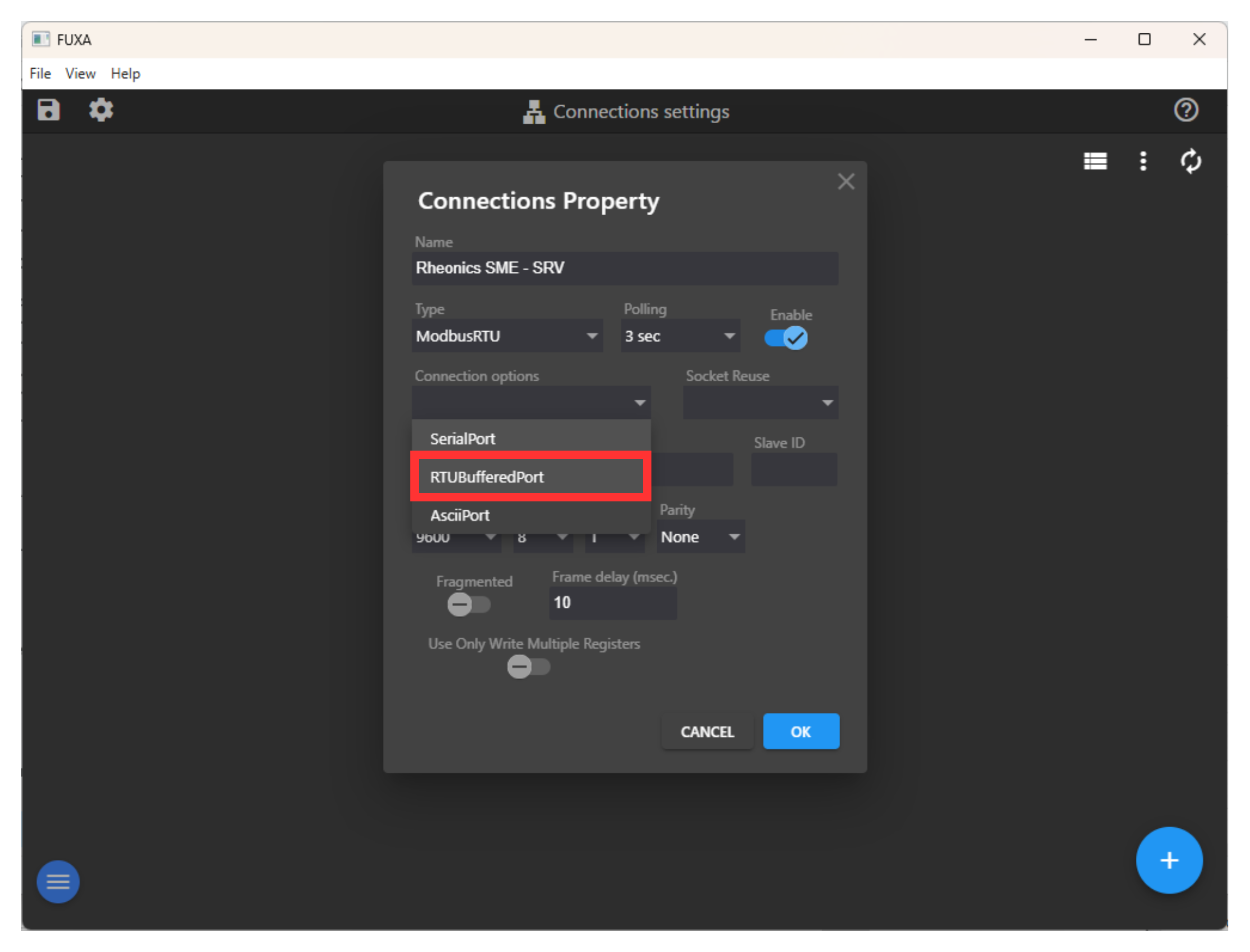
- Select RTU Buffered Port in the Connection options menu.
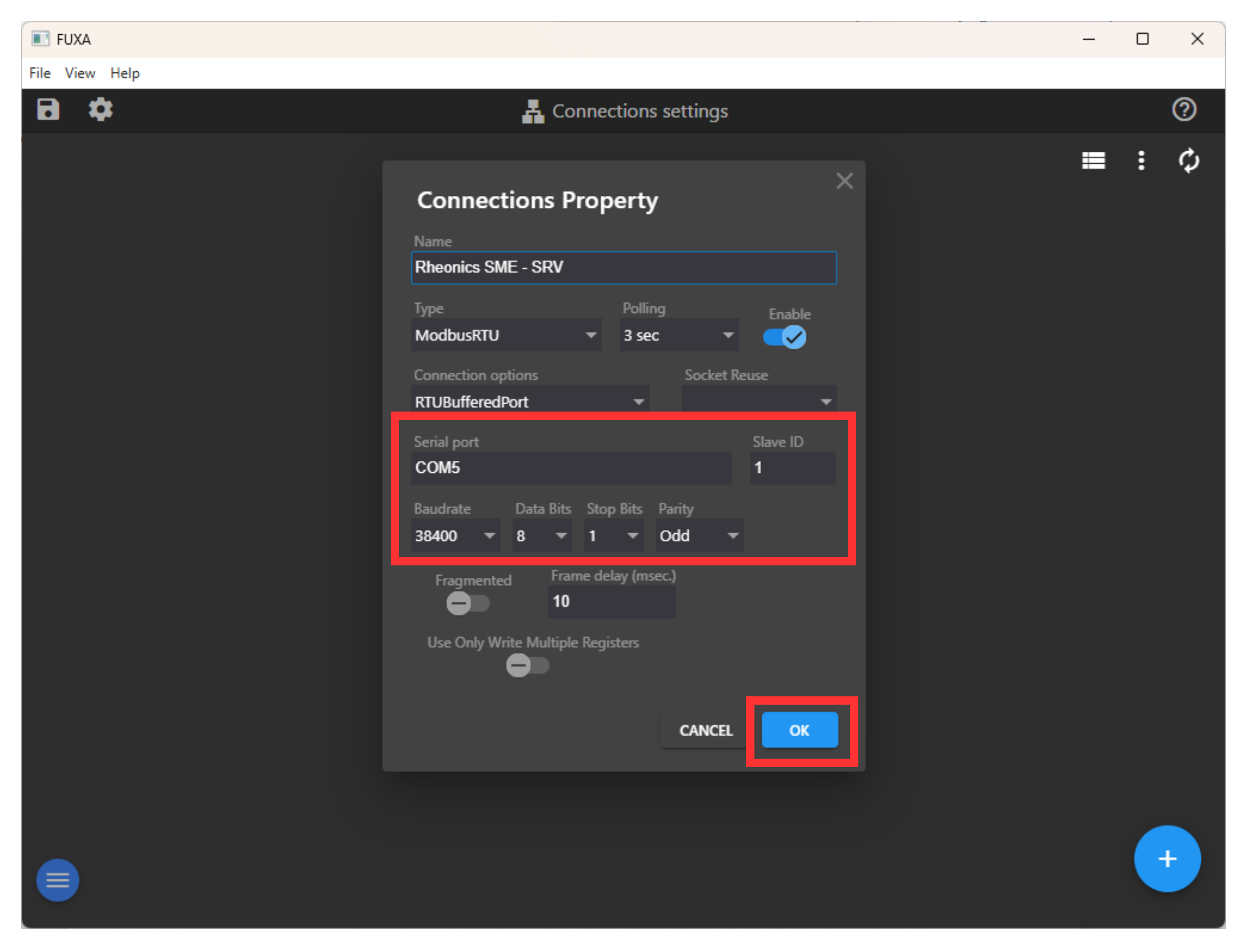
- Configure the Modbus RTU parameters according to the Connecting Modbus RTU (RS-485) outputs article.
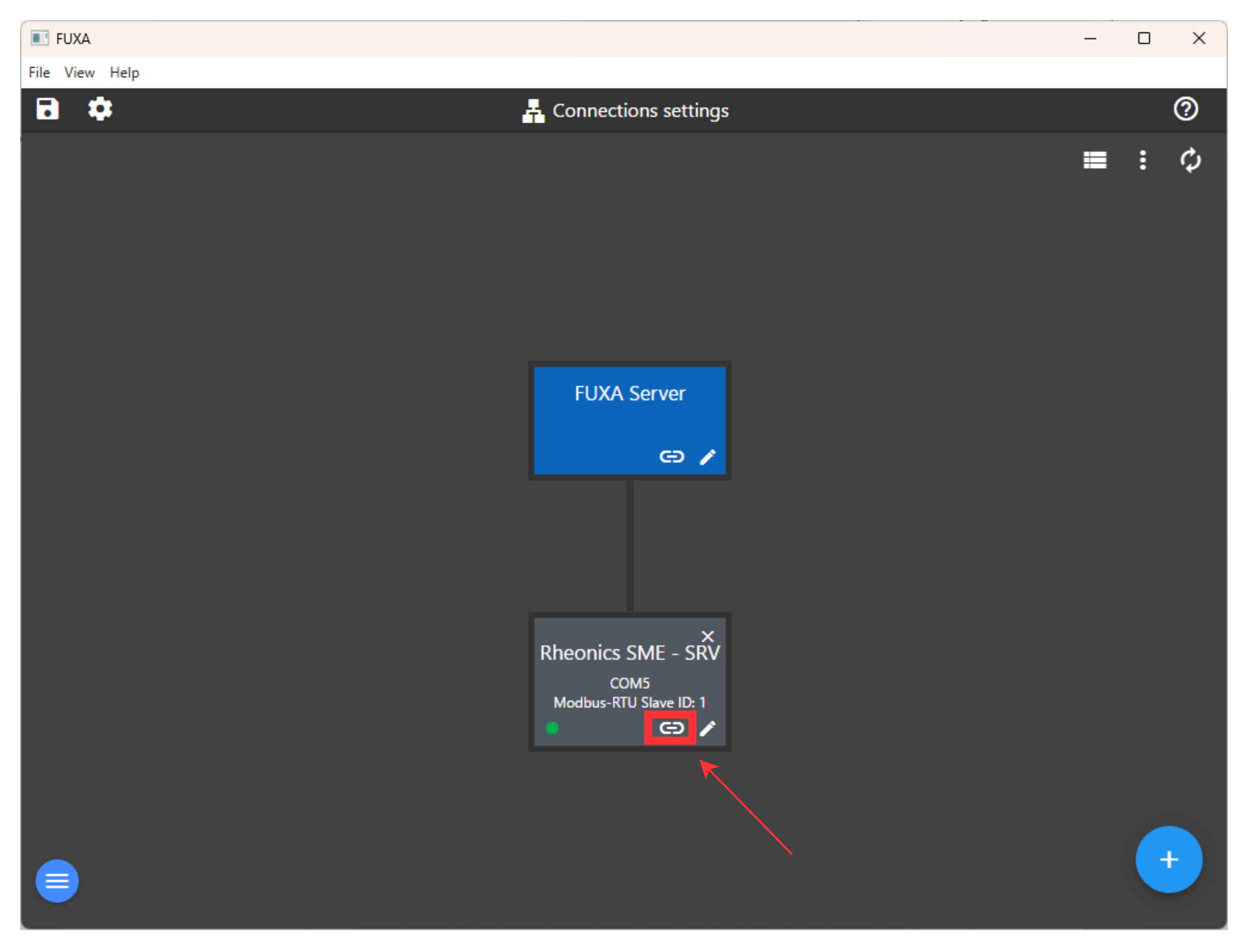
- Click on the Settings button of the Modbus block and add a new variable.
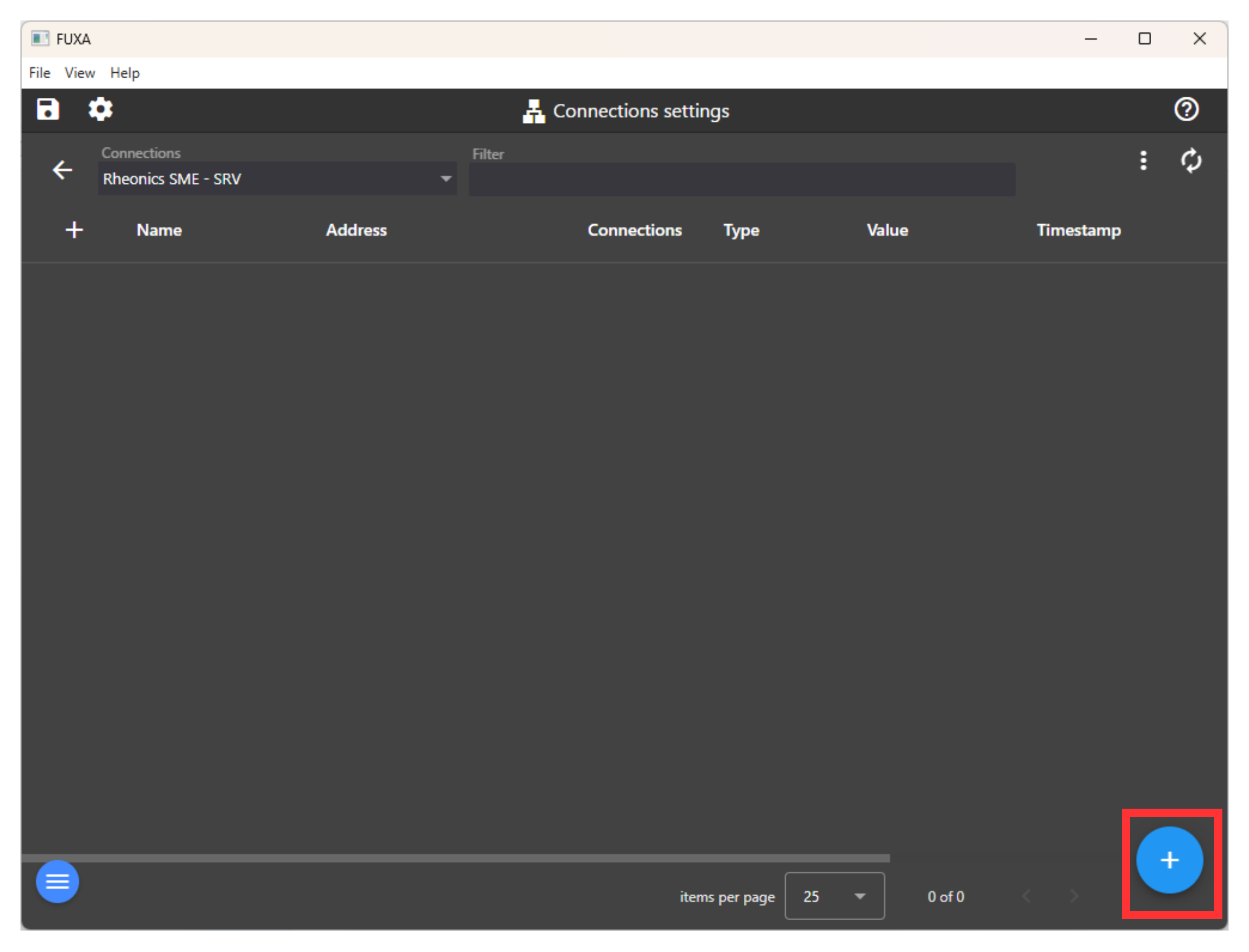
- Add the register parameters of the desired value according to the Modbus Input Registers support article.
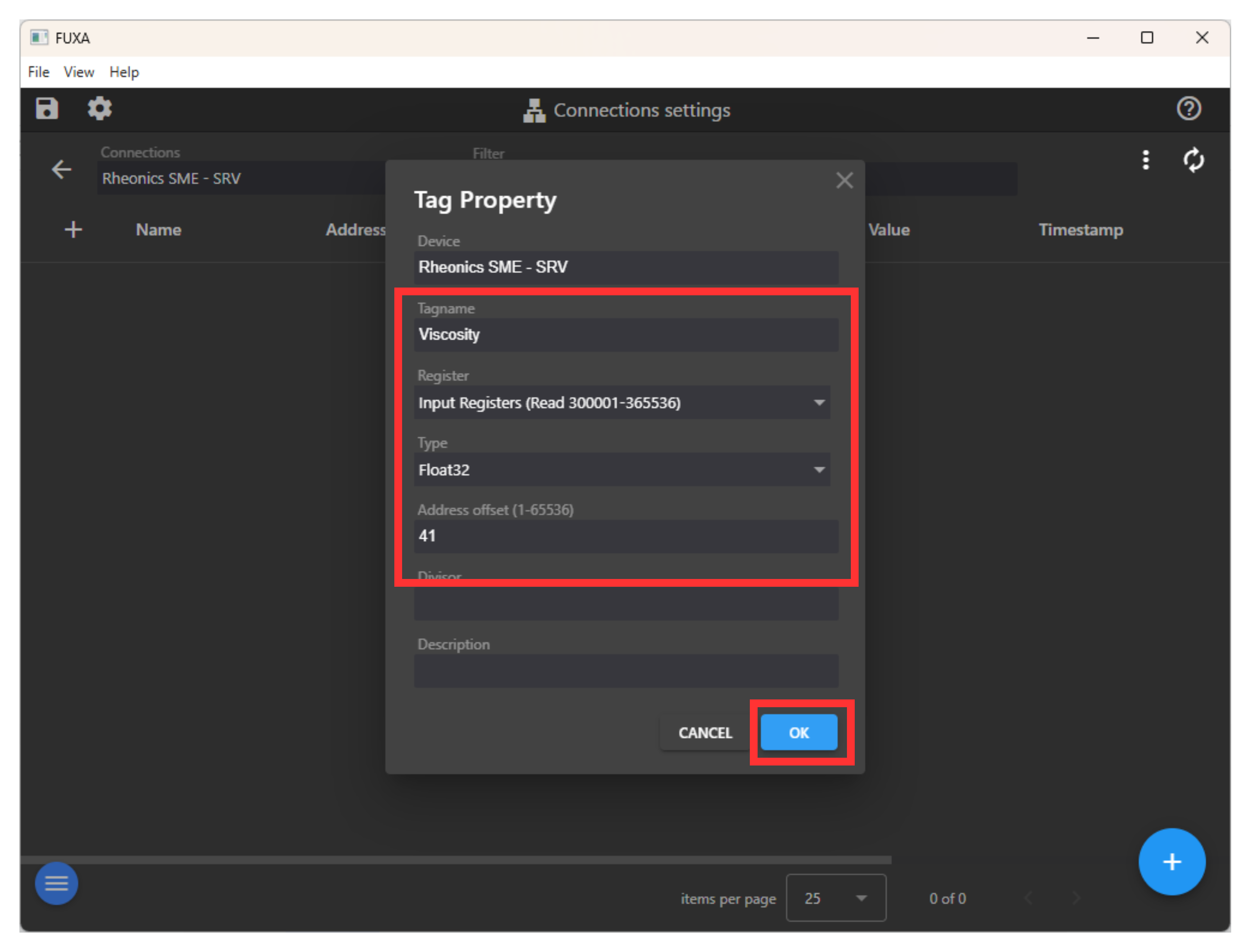
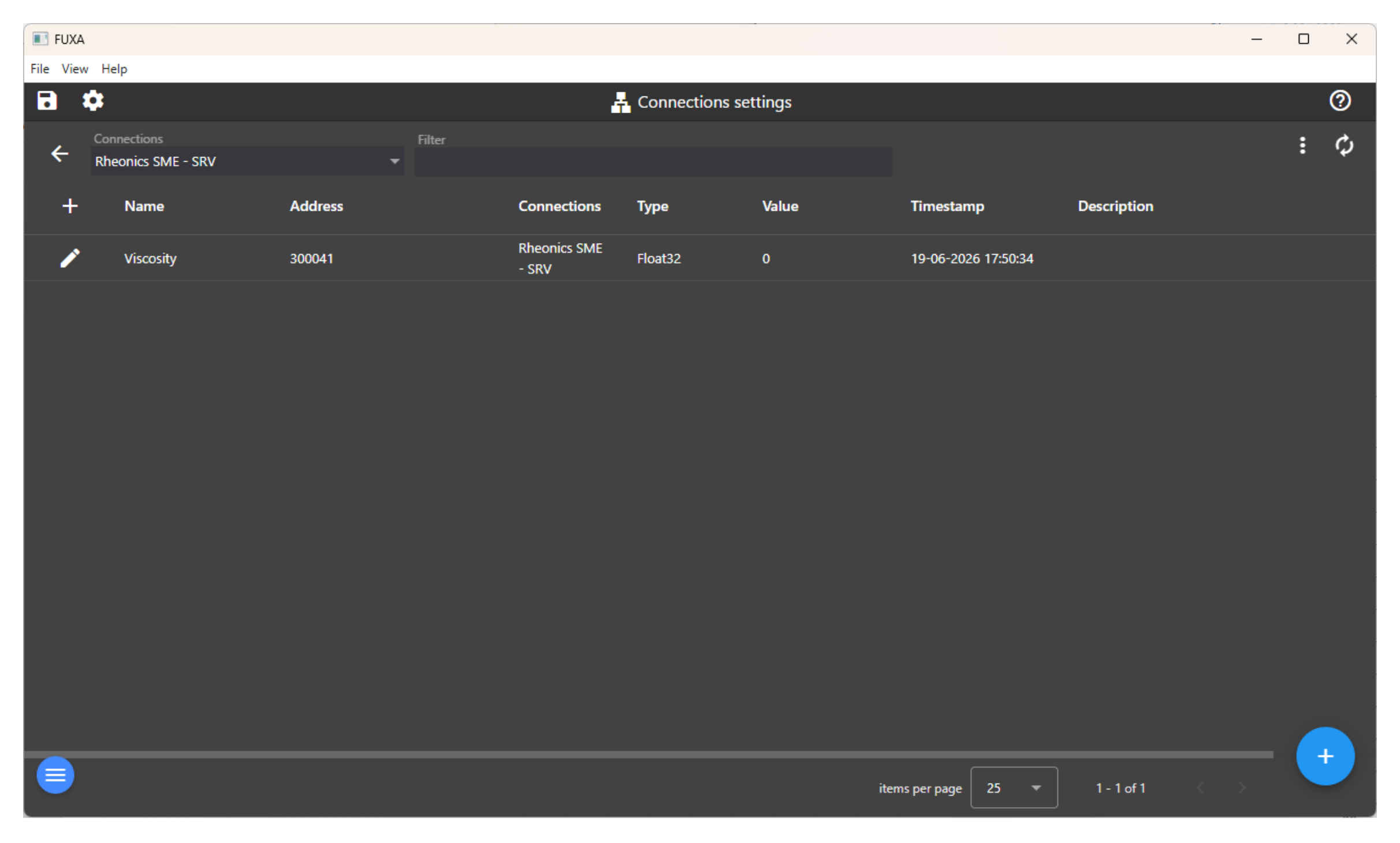
- If the parameter is correctly requested, the value and timestamp will be shown in the window.
3.2 Adding variables in Editor
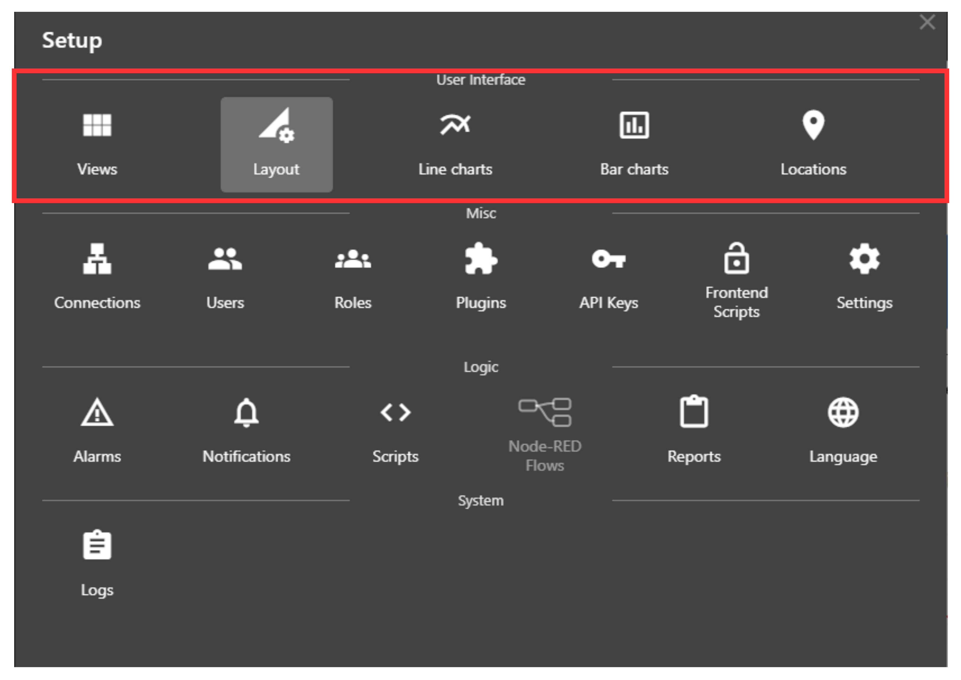
Once the blank board appears, a simple way to add variables in the project editor is by using plots. In the general settings menu, the User Interface section offers two types of charts: line plot and bar plot.
Another way is by using the side menu in the Controls section. Here you will find chart options and other control menus, such as adding output and input values, tables, images, pie charts, and animations like the Pipe option.
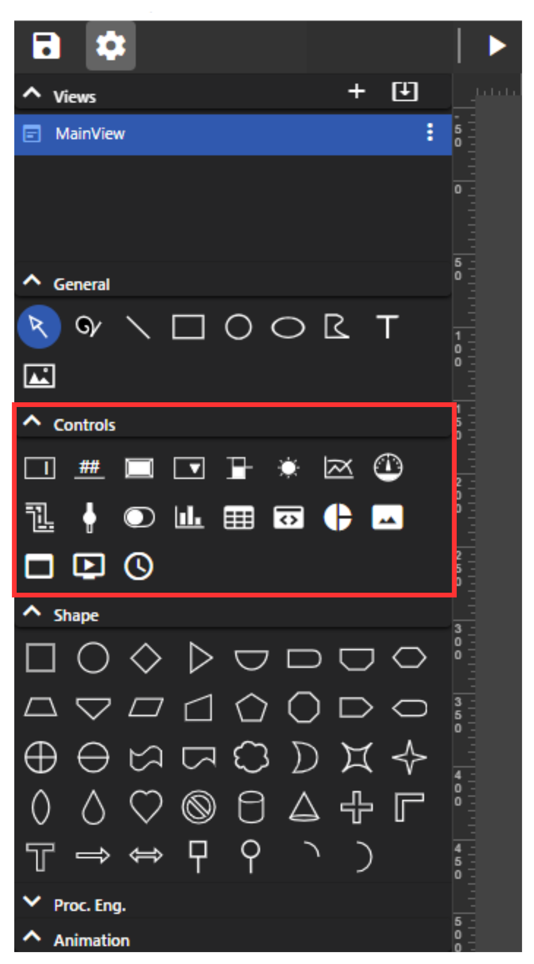
First, add a chart and give it a name. Then, select the Add Line option. In this menu, select the parameter that was added in the previous section of this article.
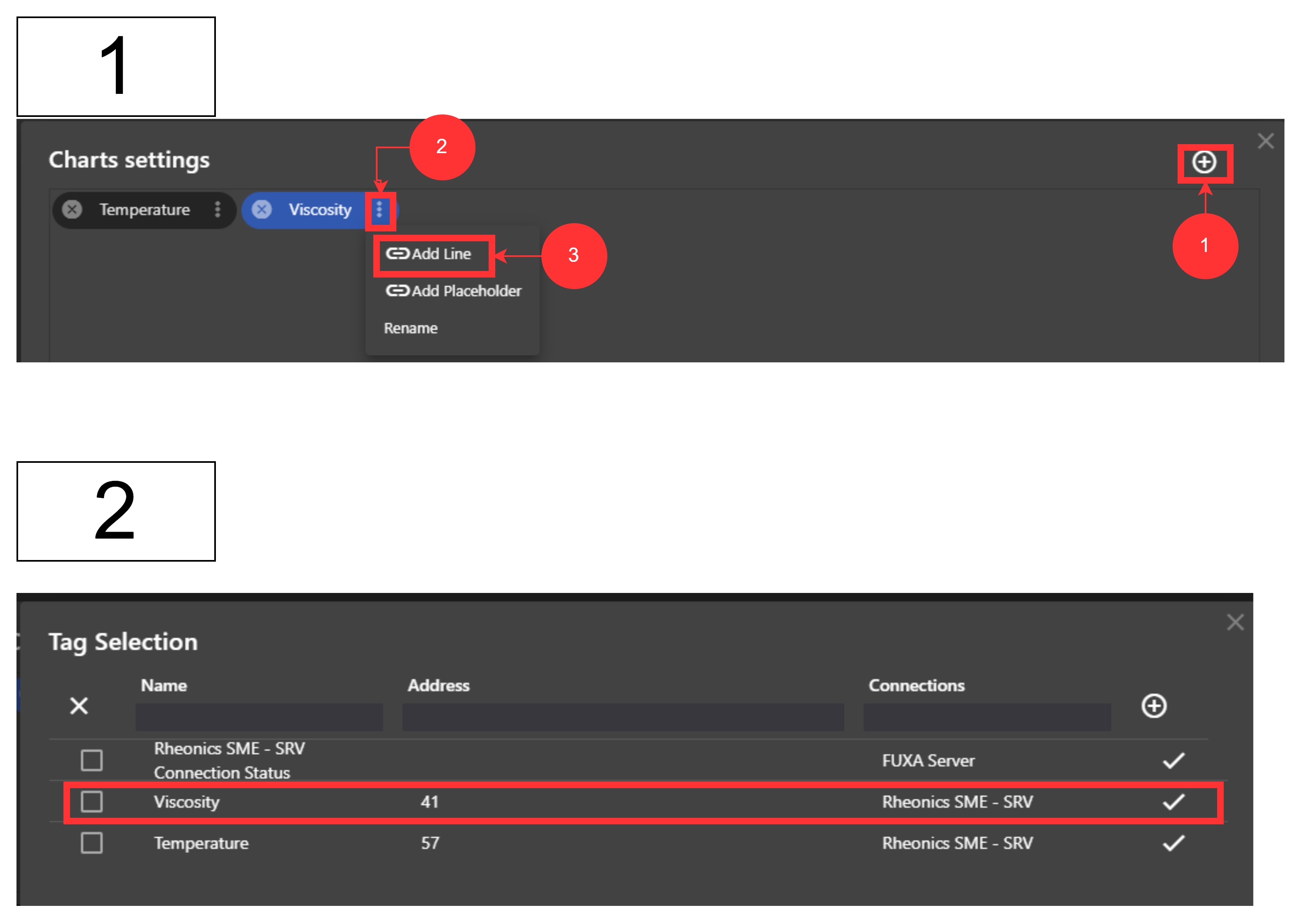
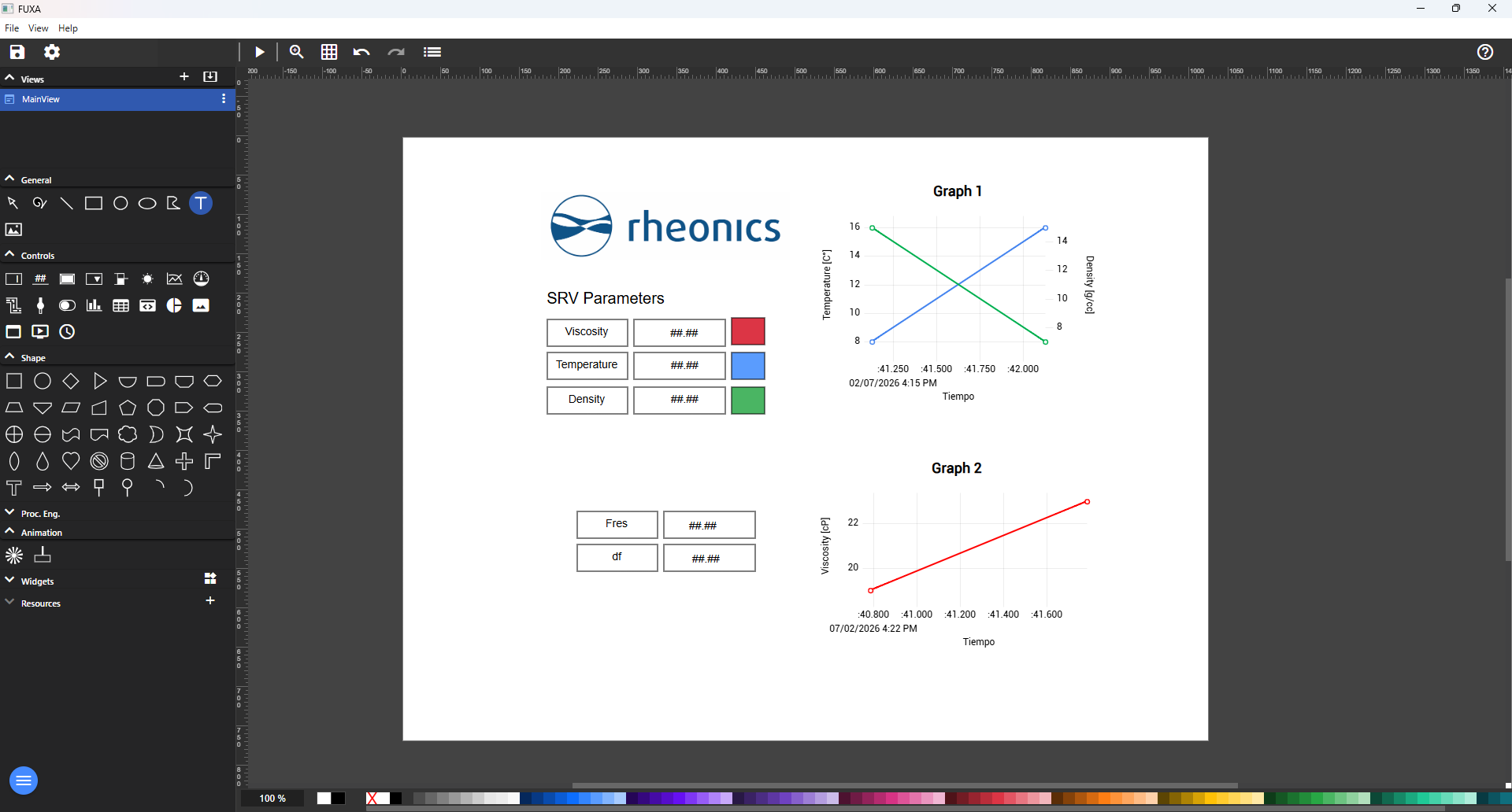
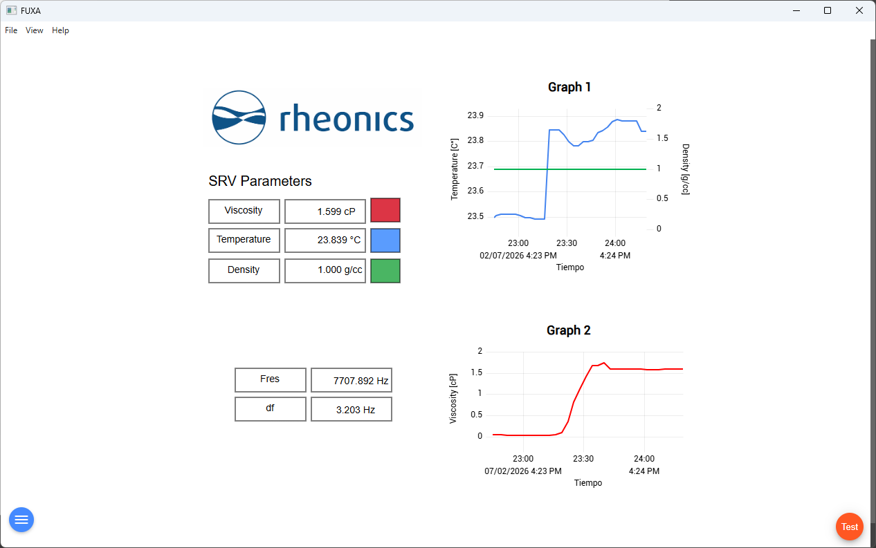
This process can be repeated depending on how many variables you want to add to the canvas and the type of representation you choose, whether real-time graphs or animations. Figures 12 and 13 show a simple example consisting of two line graphs and a display of the numerical values. The graphs display the real-time values of the selected parameters. Animations can also be configured to react to events by defining conditionals based on parameter values, allowing the interface to reflect changes in the system dynamically.
To verify that your project is functioning correctly, switch the Editor view to the Lab view. If the Lab view runs without errors, communication with the SME parameters has been successfully established, and the configured visualizations should update according to the incoming data. This confirms that both the parameter mapping and the visualization logic have been configured correctly.
Further information
Communication protocols
- Connecting Modbus RTU (RS-485) outputs — how to wire and configure the SME for Modbus RTU communication.
- Connecting the Modbus TCP outputs — setup steps for Modbus TCP/IP communication with the SME.
- Modbus Input Registers — reference list of register addresses for reading sensor parameters.
- HiveMQ broker integration with Rheonics — connecting an SME to an MQTT broker.
- Integrating Rheonics sensors with OPC UA via Modbus TCP gateway — using an OPC UA gateway with the SME.
- Rheonics sensor integration with S7-300 and Profinet — connecting the SME to a Siemens PLC.
- Taking the EtherNet/IP road with Rheonics SME — connecting the SME over EtherNet/IP.
SCADA integration
- Rheonics sensor integration with Ignition SCADA — connecting an SME to Ignition SCADA via OPC UA.
- Benefits of using Rheonics sensors with Ignition SCADA for remote monitoring — overview of remote data acquisition and visualization use cases.
References
- [1] FUXA – open-source SCADA/HMI project — github.com/frangoteam/fuxa